Intro to Dynamic Neural Networks and DyNet
By Hao Zhang
Deep learning (DL), which refers to a class of neural networks (NNs) with deep architectures, powers a wide spectrum of machine learning tasks and is correlated with state-of-the-art results. DL is distinguished from other machine learning (ML) algorithms mainly by its use of deep neural networks, a family of ML models with many interconnected layers, each composed of various mathematical operations (e.g. +, -, convolution, matmul).
Before a DL model can give predictions, it is usually trained by stochastic gradient descent (or variants) — an iterative process in which gradients are calculated through back-propagation. At each iteration of the process, a chunk of input data (e.g. images of birds in Figure 1), usually represented as a multidimensional array (tensor), is forwarded through the network following its layered structure, and then backward in reverse to compute the parameter updates.
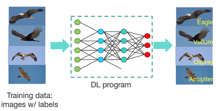

This happens repeatedly until the model parameters have been updated to some state that is regarded as optimal. Figure 2 abstracts this forward-backward process as grey blocks and arrows.
One reason for the widespread adoption of DL is the variety and quality of software toolkits, such as Caffe and TensorFlow, that ease the programming of DL models and speed computation by harnessing modern computing hardware (e.g. GPUs), software libraries (e.g. CUDA, cuDNN), and compute clusters. One dominant programming paradigm adopted by these types of DL toolkits is the representation of a neural network as a static dataflow graph (Figure 3).
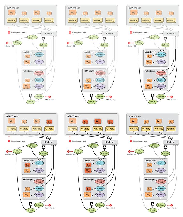
To see this, first observe that there is a natural connection between NNs and directed graphs: we can map the graph nodes to the computational operations or parameters in NNs and let the edges indicate the direction of the data being passed between the nodes. In this case, we can represent the process of training NNs as batches of data flowing through computational graphs, i.e. dataflow graphs.

This programming paradigm requires DL programmers to define the network architecture (i.e. the dataflow graph) once using symbolic expressions before beginning execution. Then, for a given graph and data samples, the software toolkits can automatically derive the correct algorithm for training or inference following backpropagation and auto-differentiation rules (Figure 4).
In the following pseudo code, I’ve summarized the workflow of this programming paradigm as “static declaration”.

With proper optimization, the execution of these static dataflow graphs can be highly efficient; as the dataflow graph is fixed for all data, the evaluation of multiple samples through one graph can be naturally batched (that is why the input to $D$ is a batch of $K$ samples $\{x_i^t\}_{i=1}^K$ instead of one single sample $x$), leveraging the improved parallelization capability of modern hardware (e.g. GPUs). Moreover, by separating model declaration and execution, it’s possible to optimize the graph at declaration time, with these optimizations benefiting the efficiency of processing arbitrary input data batches at execution time.
While the dataflow graph has major efficiency advantages, its applicability relies on a key assumption — that the graph (i.e. NN architecture) is fixed throughout the runtime. This assumption, however, breaks for dynamic NNs such as NNs that compute over sequences of variable lengths, trees, and graphs, where the network architectures conditionally change with every input sample.
Dynamic Neural Networks: An Example
Successful NN models generally exhibit suitable architectures that capture the structures of the input data. For example, convolutional neural networks (CNNs), which apply fixed-structured operations to fixed-sized images (Figure 1), are highly effective precisely because they capture the spatial invariance common in computer vision domains. However, apart from images, many forms of data are structurally complex and cannot be readily captured by fixed-structured NNs.
Appropriately reflecting these structures in the NN design has shown effective in problems in many domains, such as sentiment analysis, semantic similarity between sentence pairs, and image segmentation.
Let’s take a look at the constituency parsing problem as an example (Figure 5).
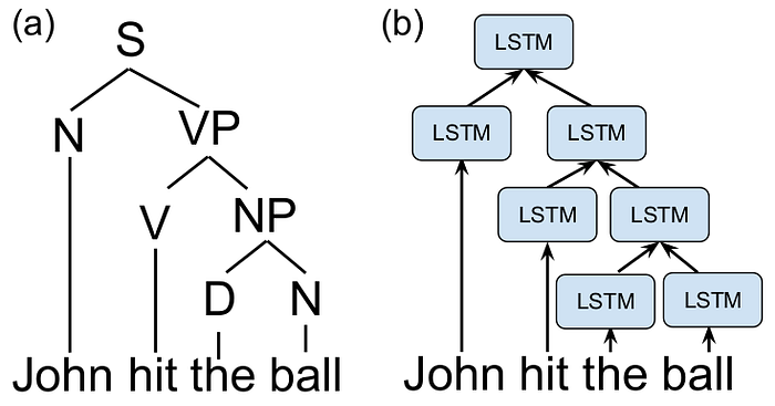
Sentences in natural languages are often represented by their constituency tree, whose structure varies depending on the content of the sentence itself (Figure 5). Constituency parsing is an important problem in natural language processing (NLP) that aims to determine the corresponding grammar type of all internal nodes given the parsing tree of a sentence.
The above figure shows an example of a network that takes into account this syntactic structure, generating representations for the sentence by traversing the parse tree bottom-up and combining the representations for each sub-tree using a dynamic NN called Tree Structured Long Short-term Memory (Tree-LSTM). Each node of the tree maps to a LSTM function. The internal computations and parameters of the LSTM function can be found in this paper, and here is a good reading to understand LSTM.
Each node takes a variable number of inputs and returns a vector representing the parsing semantics up to that point back to the leaf node. This goes on until the root LSTM node returns a vector representing the semantics of the entire sentence.
It’s important to observe that the NN structure varies with the underlying parsing tree over each input sample, but the same LSTM cell (i.e. the parametrization point of the model) is constant in shape and repeated at each internal node. Similar examples can be found for graph input and sequences of variable lengths. We refer to these NNs that exhibit different structures for different input samples as dynamic neural networks, in contrast to the static networks that have fixed network architecture for all samples.
“Static” Declaration for “Dynamic” NNs
Mentioned previously, static declaration is one dominant programming paradigm for NNs. As the static dataflow graph assumption no longer holds for dynamic structures, static declaration, using a single dataflow graph $\mathcal{D}$, cannot express dynamic NNs with structures changing with data samples. A primary remedy to this problem is to expand the symbolic programming language to allow it to explicitly include the control structure necessary to implement these applications:
Static unrolling is a standard way to express sequence recurrent NNs with fixed steps. To handle variable-length data, it declares a recurrent neural network (RNN) that has a number of steps equal to the length of the longest sequence in the dataset. It then appends zeros at the end of other sequences to have equal length, and feeds them in batches to the dataflow graph for computation. This technique costs unnecessary computation to process shorter sequences.
Bucketing improves over static unrolling — instead of padding all inputs to be the same size, it buckets them according to their length (sequences that are not bucketable are zero-padded to fit into the nearest bucket). It then creates a fixed-step RNN (i.e. a dataflow graph) for each bucket, and performs batched computation therein. Compared to static unrolling, bucketing saves considerable computation, but introduces a bucketing process that adds extra complexity.
Both static unroll and bucketing pad with zeros at the ends of samples so that they have the same structure (i.e. same length) for batched computation. However, they both result in unnecessary computation and cannot express structures that are more complex than sequences. The major obstacle preventing static declaration from being applied to express dynamic networks, is that a single dataflow graph cannot express dynamic-varying NN structures.
Dynamic Declaration
This is where DyNet comes in. In contrast to many early frameworks such as Caffe, TensorFlow, or MxNet, DyNet adopts a slightly different programming paradigm called Dynamic Declaration, which is illustrated below:
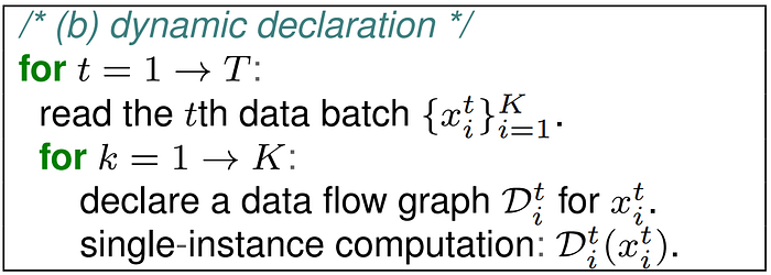
By creating a unique dataflow graph $\mathcal{D}_i^t$ for each sample $x_i^t$ according to its associated structure, dynamic declaration is able to express sample-dependent dataflow graphs. As a programming model, dynamic declaration is compatible with most DL frameworks as it demands little change on low-level implementations of the original framework.
That being said, frameworks like TensorFlow or MxNet by nature are amendable to dynamic declaration, as long as the programmers are willing to program a dataflow graph for each sample-dependent structure (e.g. parsing trees).
If you take a second look at the above pseudo code, you’ll notice that:
- Constructing a dataflow graph is not free — it will have some overhead. Since a dataflow graph $\mathcal{D}_i^t$ needs to be constructed per sample, the overhead linearly increases with the number of samples and this sometimes yields downgraded performance. This problem can be observed in frameworks like TensorFlow where creating a dataflow graph per sample takes 70% of the overall running time.
- More importantly, where in static declaration the dataflow computation $\mathcal{D}$ is applied to a batch of training samples ($\mathcal{D}{\{x_i^t\}_{i=1}^K}$ in Figure 5), in dynamic declaration, we are unable to batch the computation of differently structured graphs. Instead, only single-instance computation (\mathcal{D}_{k}^p(x_k^p)), showed in the last line of the above figure, could be performed, which would be very inefficient in the absence of batched computation.
DyNet, as a second generation DL framework, attempts to address these two challenges.
DyNet and Dynamic Batching
DyNet addresses the first challenge in a very simple way — unlike frameworks like TensorFlow, which are created for static dataflow graphs and thus ignore the overhead of graph construction, DyNet puts substantial effort into optimizing the graph construction in the framework to be lightweight, fast, and very efficient. An empirical comparison shows that DyNet’s graph construction time only takes 10% of the overall running time when training an LSTM language model (which is one of the most widely adopted dynamic NNs). You can refer to DyNet code for more details on this.
In order to address the second challenge, DyNet has to make a few innovations. I’m going to focus on one of them, called dynamic batching.
Batched Computation
Modern CPUs and GPUs evaluate batches of arithmetic operations significantly faster than the sequential evaluation of the same operations. For example, performing elementwise operations takes nearly the same amount of time on a GPU whether it’s operating on tens or on thousands of elements. Multiplying a few hundred different vectors by the same matrix is significantly slower than executing a single (equivalent) matrix-matrix product using an optimized GEMM implementation on either a GPU or a CPU. Many believe that this property of modern hardware is one of the major reasons deep learning is so successful.
In some cases, this batching is easy: when inputs and outputs are naturally represented as fixed sized tensors (e.g. images of a fixed size such as those in Figure 1), and the computations required to process each instance are instance-invariant and expressible as standard operations on tensors (e.g. a series of matrix multiplications, convolutions, and elementwise nonlinearities). For example, by adding a leading or trailing dimension to the tensors representing inputs and outputs, the developer can write code for the computation on an individual instance and pack several instances into a tensor as a “minibatch”. A suitable tensor computation library can efficiently execute these in parallel.
Unfortunately, this idealized scenario breaks when working with more complex architectures. For example, data structured as trees (Figure 5) or graphs, or selection of a different computation conditional on the input by the model. In all these cases, while the desired computation is easy enough to write for a single instance, organizing the computational operations so that they make optimally efficient use of the hardware is nontrivial. Thus, careful grouping of operations from different structured graphs into batches that can execute efficiently in parallel is crucial for making the most of available hardware resources. In this context, we call these grouping procedures “dynamic batching”.
Dynamic Batching
DyNet is the first framework to perform dynamic batching in dynamic declaration. DyNet proposed/adopted two smart methods to find available operations that can be batched together: depth-based batching and agenda-based batching (Figures 6 & 7).
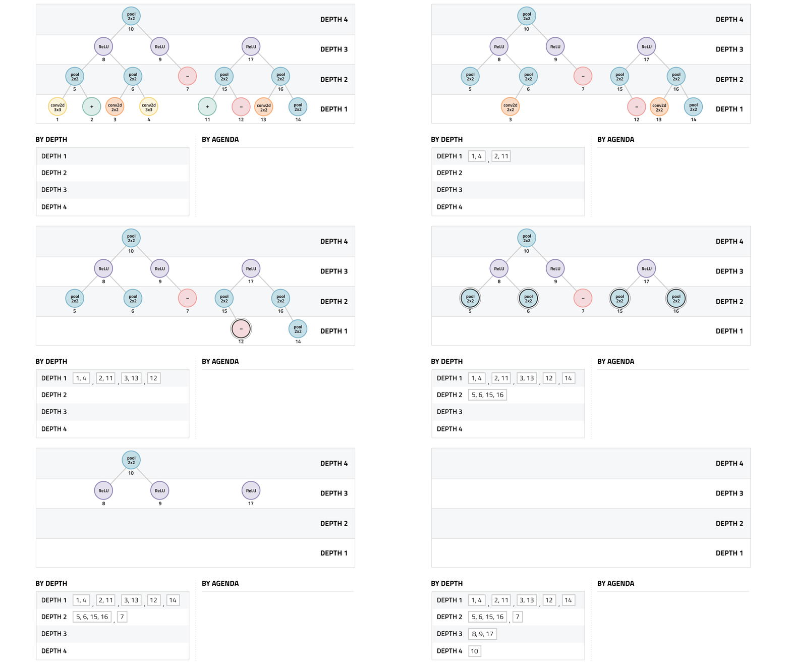

Depth-based batching is done by calculating the depth of each node in the original computation graph, defined as the maximum length from a leaf node to the node itself, and batching together nodes that have an identical depth and signature. By construction, nodes of the same depth are not dependent on each other, as all nodes have a higher depth than their input. Thus, this batching strategy is guaranteed to be viable.
Agenda-based batching is a method that does not depend solely on depth. The core of this method is an agenda that tracks “available” nodes that have no unresolved dependencies. A count of each node’s unresolved dependencies is maintained and initialized to be the number of inputs to the node. The agenda is initialized by adding nodes that have no incoming inputs (and thus no unresolved dependencies). At each iteration, we select a node from the agenda together with all of the available nodes in the same signature, and group them into a single batch operation. These nodes are then removed from the agenda, and the dependency counters of all of their successors are decremented. Any new zero-dependency nodes are added to the agenda and this process is repeated until all nodes have been processed.
While I use two very simple examples to illustrate these ideas, DyNet’s dynamic batching is in practice way more complex. Different batching strategies have different pros and cons, and it’s also important to consider other problem areas such as checking signatures, guaranteeing memory continuity, and scheduling computational kernels. For more details, I recommend to taking a look at this paper and DyNet code.
How effective is dynamic batching based on the above two strategies?

Figure 7 compares the TensorFlow Fold, a former state-of-the-art framework for dynamic NNs, to DyNet dynamic batching on training the TreeLSTM with the Stanford Sentiment Treebank dataset. In terms of how many trees can be processed per second, the DyNet performance is better across the board stratified by hardware type — it is consistently 2–4 times faster.
Furthermore, DyNet has greater throughput on CPU than TensorFlow Fold on GPU until batch sizes exceed 64. With single instance training, DyNet’s sequential evaluation processes 46.7 trees/second on CPU, whereas autobatching processes 93.6 trees/second. This demonstrates that in complex architectures like TreeLSTMs, there are opportunities to batch up operations inside a single training instance, which are exploited by the dynamic batching algorithm.
Future reading
Due to the growing interest in these sorts of dynamic models, recent years have seen an increase in the popularity of frameworks based on dynamic declaration. DyNet is among the best of them, but it’s not able to address all of the problems that we experience in dynamic neural networks.
If you are interested in more advanced techniques for dynamic neural networks, I recommend the following readings:
- Cavs: A Vertex-centric Programming Interface for Dynamic Neural Networks
- Deep Learning with Dynamic Computation Graphs
- On-the-fly Operation Batching in Dynamic Computation Graphs
And don’t forget to give DyNet code a try! It’s open sourced here: http://dynet.io/
